Discussion on HackerNews

Diffusion models have recently produced impressive results in generative modeling, in particular sampling from multimodal distributions. Not only has diffusion models seen widespread adoption in text-to-image generation tools such as Stable Diffusion, they also excel in other application domains such as audio/video/3D generation, protein design, robotics path planning, all of which require sampling from multimodal distributions.

This tutorial aims to introduce diffusion models from an optimization perspective as introduced in our paper (joint work with Frank Permenter). It will go over both theory and code, using the theory to explain how to implement diffusion models from scratch. By the end of the tutorial, you will learn how to implement training and sampling code for a toy dataset, which will also work for larger datasets and models.

In this tutorial we will mainly reference code from smalldiffusion. For pedagogical purposes, the code presented here will be simplified from the original library code, which is on its own well-commented and easy to read.

Training diffusion models

Diffusion models aim to generate samples from a set that is learned from training examples, which we will denote by \(\mathcal{K}\). For example, if we want to generate images, \(\mathcal{K} \subset \mathbb{R}^{c\times h \times w}\) is the set of pixel values that correspond to realistic images. Diffusion models also work for \(\mathcal{K}\) corresponding to modalities other than images, such as audio, video, robot trajectories, and even in discrete domains such as text generation.

In a nutshell, diffusion models are trained by:

1. Sampling \(x_0 \sim \mathcal{K}\), noise level \(\sigma \sim [\sigma_\min, \sigma_\max]\), noise \(\epsilon \sim N(0, I)\)
2. Generating noisy data \(x_\sigma = x_0 + \sigma \epsilon\)
3. Predicting \(\epsilon\) (direction of noise) from \(x_\sigma\) by minimizing squared loss

This amounts to training a \(\theta\)-parameterized neural network \(\epsilon_\theta(x, \sigma)\), by minimizing the loss function

In practice, this is done by the following simple training_loop:

def training_loop(loader  : DataLoader,
                  model   : nn.Module,
                  schedule: Schedule,
                  epochs  : int = 10000):
    optimizer = torch.optim.Adam(model.parameters())
    for _ in range(epochs):
        for x0 in loader:
            optimizer.zero_grad()
            sigma, eps = generate_train_sample(x0, schedule)
            eps_hat = model(x0 + sigma * eps, sigma)
            loss = nn.MSELoss()(eps_hat, eps)
            optimizer.backward(loss)
            optimizer.step()

The training loop iterates over batches of x0, then samples noise level sigma and noise vector eps using generate_train_sample:

def generate_train_sample(x0: torch.FloatTensor, schedule: Schedule):
    sigma = schedule.sample_batch(x0)
    eps = torch.randn_like(x0)
    return sigma, eps

Noise schedules

In practice, \(\sigma\) is not sampled uniformly from the interval \([\sigma_\min, \sigma_\max]\), instead this interval is discretized into \(N\) distinct values called a \(\sigma\) schedule: \(\{ \sigma_t \}_{t=1}^N\), and \(\sigma\) is instead sampled uniformly from the \(N\) possible values of \(\sigma_t\). We define the Schedule class that encapsulates the list of possible sigmas, and sample from this list during training.

class Schedule:
    def __init__(self, sigmas: torch.FloatTensor):
        self.sigmas = sigmas
    def __getitem__(self, i) -> torch.FloatTensor:
        return self.sigmas[i]
    def __len__(self) -> int:
        return len(self.sigmas)
    def sample_batch(self, x0:torch.FloatTensor) -> torch.FloatTensor:
        return self[torch.randint(len(self), (x0.shape[0],))].to(x0)

In this tutorial, we will use a log-linear schedule defined below:

class ScheduleLogLinear(Schedule):
    def __init__(self, N: int, sigma_min: float=0.02, sigma_max: float=10):
        super().__init__(torch.logspace(math.log10(sigma_min), math.log10(sigma_max), N))

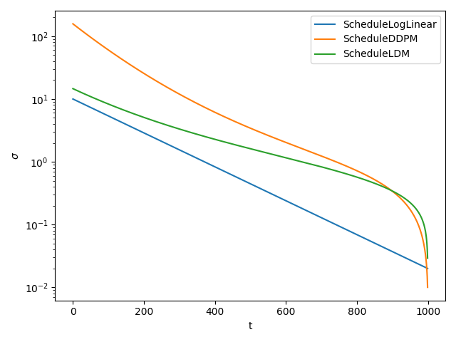
Other commonly used schedules include ScheduleDDPM for pixel-space diffusion models and ScheduleLDM for latent diffusion models such as Stable Diffusion. The following plot compares these three schedules with default parameters.

Toy example

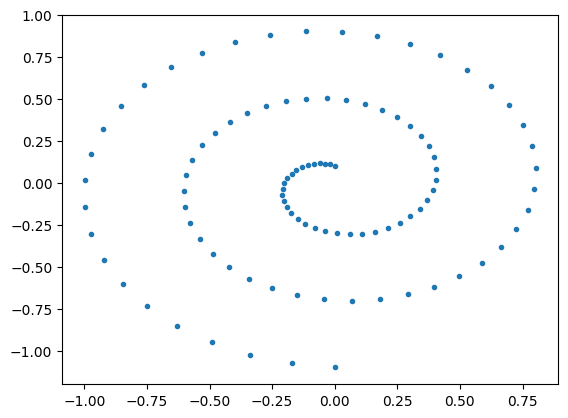
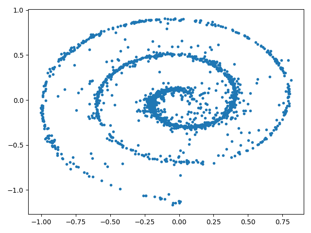
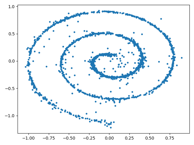
In this tutorial we will start with a toy dataset used in one of the first diffusion papers [Sohl-Dickstein et.al. 2015], where \(\Kset \subset \R^2\) are points sampled from a spiral. We first construct and visualize this dataset:

dataset = Swissroll(np.pi/2, 5*np.pi, 100)
loader  = DataLoader(dataset, batch_size=2048)

For this simple dataset, we can implement the denoiser using a multi-layer perceptron (MLP):

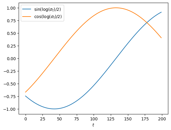
def get_sigma_embeds(sigma):
    sigma = sigma.unsqueeze(1)
    return torch.cat([torch.sin(torch.log(sigma)/2),
                      torch.cos(torch.log(sigma)/2)], dim=1)

class TimeInputMLP(nn.Module):
    def __init__(self, dim, hidden_dims):
        super().__init__()
        layers = []
        for in_dim, out_dim in pairwise((dim + 2,) + hidden_dims):
            layers.extend([nn.Linear(in_dim, out_dim), nn.GELU()])
        layers.append(nn.Linear(hidden_dims[-1], dim))
        self.net = nn.Sequential(*layers)
        self.input_dims = (dim,)

    def rand_input(self, batchsize):
        return torch.randn((batchsize,) + self.input_dims)

    def forward(self, x, sigma):
        sigma_embeds = get_sigma_embeds(sigma)         # shape: b x 2
        nn_input = torch.cat([x, sigma_embeds], dim=1) # shape: b x (dim + 2)
        return self.net(nn_input)

model = TimeInputMLP(dim=2, hidden_dims=(16,128,128,128,128,16))

The MLP takes the concatenation of \(x \in \R^2\) and an embedding of the noise level \(\sigma\), then predicts the noise \(\epsilon \in \R^2\). Although many diffusion models use a sinusoidal positional embedding for \(\sigma\), the simple two-dimensional embedding works just as well:

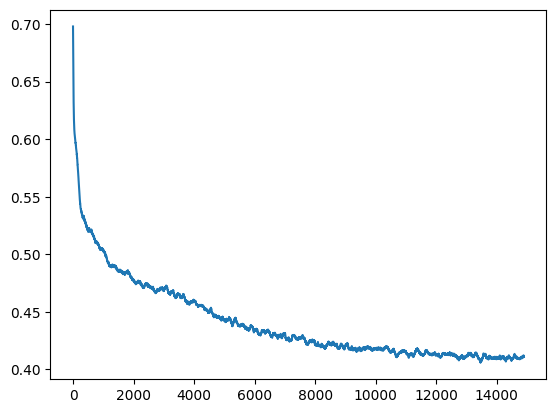
Now we have all the ingredients to train a diffusion model.

schedule = ScheduleLogLinear(N=200, sigma_min=0.005, sigma_max=10)
trainer  = training_loop(loader, model, schedule, epochs=15000)
losses   = [ns.loss.item() for ns in trainer]

The learned denoiser \(\eps_\theta(x, \sigma)\) can be visualized as a vector field parameterized by the noise level \(\sigma\), by plotting \(x - \sigma \eps_\theta(x, \sigma)\) for different \(x\) and levels of \(\sigma\).

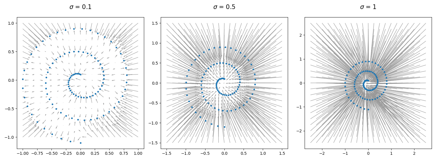
In the plots above, the arrows point from each noisy datapoint \(x\) to the “clean” datapoint predicted by the denoiser with noise level \(\sigma\). At high levels of \(\sigma\), the denoiser tends to predict the mean of the data, but at low noise levels the denoiser predicts actual data points, provided that its input \(x\) is also close to the data.

How do we interpret what the denoiser is learning, and how do we create a procedure to sample from diffusion models? We will next build a theory of diffusion models, then draw on this theory to derive sampling algorithms.

Denoising as approximate projection

The diffusion training procedure learns a denoiser \(\eps_\theta(x, \sigma)\). In our paper, we interpret the learned denoiser as an approximate projection to the data manifold \(\Kset\), and the goal of the diffusion process as minimizing the distance to \(\Kset\). This motivates us to introduce a relative-error approximation model to analyze the convergence of diffusion sampling algorithms. First we introduce some basic properties of distance and projection functions.

Distance and projection functions

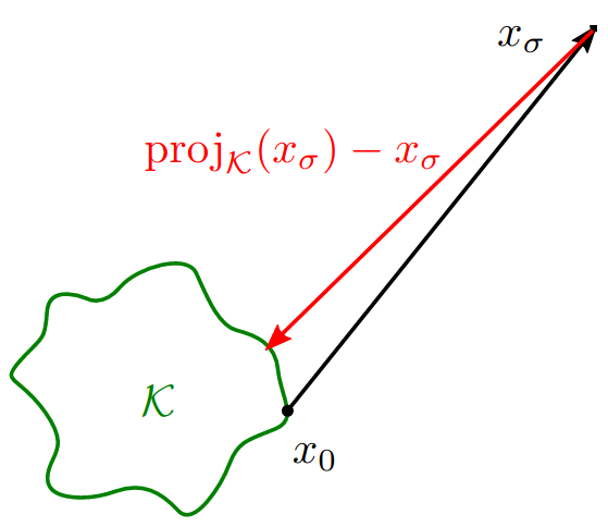
The distance function to a set \(\Kset \subseteq \R^n\) is defined as

The projection of \(x \in \R^n\), denoted \(\projK(x)\), is the set of points that attain this distance:

If \(\projK(x)\) is unique, the gradient of \(\distK(x)\), the direction of steepest descent of the distance function, points towards this unique projection:

Proposition Suppose \(\Kset\) is closed and \(x \not \in \Kset\). If \(\projK(x)\) is unique, then

This tells us that if we can learn \(\nabla \distK(x)\) for every \(x\), we can simply move in this direction to find the projection of \(x\) onto \(\Kset\). One issue with learning this gradient is that \(\distK\) is not differentiable everywhere, thus \(\nabla \distK\) is not a continuous function. To solve this problem, we introduce a squared-distance function smoothed by a parameter \(\sigma\) using the \(\softmin\) operator instead of \(\min\).

The following picture from [Madan and Levin 2022] shows the contours of both the distance function and its smoothed version.

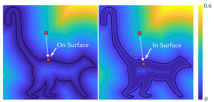
From this picture we can see that \(\nabla \distK(x)\) points toward the closest point to \(x\) in \(\Kset\), and \(\nabla \distop^2(x, \sigma)\) points toward a weighted average of points in \(\Kset\) determined by \(x\).

Ideal denoiser

The ideal or optimal denoiser \(\epsilon^*\) for a particular noise level \(\sigma\) is an exact minimizer of the training loss function. When the data is a discrete uniform distribution over a finite set \(\Kset\), the ideal denoiser has an exact closed-form expression given by:

From the above expression, we see that the ideal denoiser points towards a weighted mean of all the datapoints in \(\Kset\), where the weight for each \(x_0 \in \Kset\) determines the distance to \(x_0\). Using this expression, we can also implement the ideal denoiser, which is computationally tractable for small datasets:

def sq_norm(M, k):
    # M: b x n --(norm)--> b --(repeat)--> b x k
    return (torch.norm(M, dim=1)**2).unsqueeze(1).repeat(1,k)

class IdealDenoiser:
    def __init__(self, dataset: torch.utils.data.Dataset):
        self.data = torch.stack(list(dataset))

    def __call__(self, x, sigma):
        x = x.flatten(start_dim=1)
        d = self.data.flatten(start_dim=1)
        xb, db = x.shape[0], d.shape[0]
        sq_diffs = sq_norm(x, db) + sq_norm(d, xb).T - 2 * x @ d.T
        weights = torch.nn.functional.softmax(-sq_diffs/2/sigma**2, dim=1)
        return (x - torch.einsum('ij,j...->i...', weights, self.data))/sigma

For our toy dataset, we can plot the direction of \(\epsilon^*\) as predicted by the ideal denoiser for different noise levels \(\sigma\):

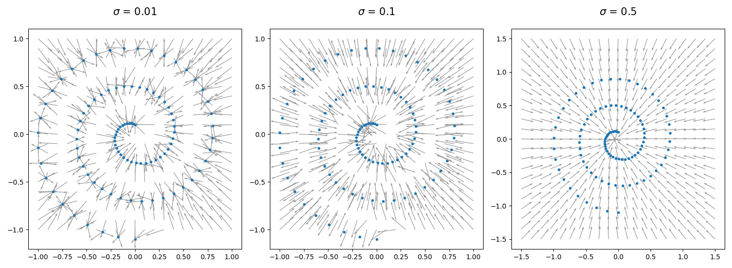
From our plots we see that for large values of \(\sigma\), \(\epsilon^*\) points towards the mean of the data, but for smaller values of \(\sigma\), \(\epsilon^*\) points towards the nearest data-point.

One insight from our paper is that the ideal denoiser for a fixed \(\sigma\) is equivalent to the gradient of a \(\sigma\)-smoothed squared-distance function:

Theorem For all \(\sigma > 0\) and \(x \in \R^n\), we have

This tells us that the ideal denoiser found by minimizing the diffusion training objective \(\Loss(\theta)\) is in fact the gradient of a smoothed squared-distance function to the underlying data manifold \(\Kset\). This connection is key to motivating our interpretation that the denoiser is an approximate projection.

Relative error model

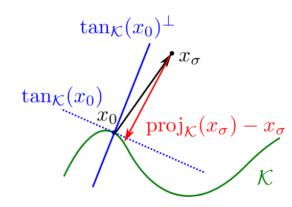
In order to analyze the convergence of diffusion sampling algorithms, we introduced a relative error model which states that the projection predicted by the denoiser \(x-\sigma \epsilon_{\theta}( x, \sigma)\) well approximates \(\projK(x)\) when the input to the denoiser \(\sigma\) well estimates \(\distK(x)/\sqrt{n}\). For constants \(1 > \eta \ge 0\) and \(\nu \ge 1\), we assume that

when \((x, \sigma)\) satisfies \(\frac{1}{\nu}\distK(x) \le \sqrt{n}\sigma \le \nu \distK(x)\). In addition to the discussion about ideal denoisers above, this error model is motivated by the following observations.

Low noise When \(\sigma\) is small and the manifold hypothesis holds, denoising approximates projection because most of the added noise is orthogonal to the data manifold.

High noise When \(\sigma\) is large relative to the diameter of \(\Kset\), then any denoiser predicting any weighted mean of the data \(\Kset\) has small relative error.

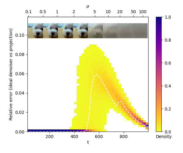
We also perform empirical tests of our error model for pre-trained diffusion models on image datasets. The CIFAR-10 dataset is small enough for tractable computation of the ideal denoiser. Our experiments show that for this dataset, the relative error between the exact projection and ideal denoiser output is small over sampling trajectories.

Sampling from diffusion models

Given a learned denoiser \(\epsilon_\theta(x, \sigma)\), how do we sample from it to obtain a point \(x_0 \in \Kset\)? Given noisy \(x_t\) and noise level \(\sigma_t\), the denoiser \(\eps_\theta(x_t, \sigma_t)\) predicts \(x_0\) via

Intuition from the relative error assumption tells us that we want to start with \((x_T, \sigma_T)\) where \(\distK(x_T)/\sqrt{n} \approx \sigma_T\). This is achieved by choosing \(\sigma_T\) to be large relative to the diameter of \(\Kset\), and \(x_T\) sampled i.i.d. from \(N(0, \sigma_T)\), a Gaussian with variance \(\sigma_T\). This ensures that \(x_T\) is far away from \(\Kset\).

Although \(\hat x_0^T = x_T - \sigma_T \eps_\theta(x_T, \sigma_T)\) has small relative error, the absolute error \(\distK(\hat x_0^T)\) can still be large as \(\distK(x_T)\) is large. In fact, at high noise levels, the expression of the ideal denoiser tells us that \(\hat x_0^T\) should be close to the mean of the data \(\Kset\). We cannot obtain a sample close to \(\Kset\) with a single call to the denoiser.

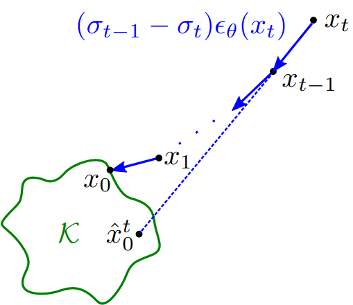
Thus we want to iteratively call the denoiser to obtain a sequence \(x_T, \ldots, x_t, \ldots x_0\) using a pre-specified schedule of \(\sigma_t\), hoping that \(\distK(x_t)\) decreases in concert with \(\sigma_t\).

This is exactly the deterministic DDIM sampling algorithm, though presented in different coordinates through a change of variable. See Appendix A of our paper for more details and a proof of equivalence.

Diffusion sampling as distance minimization

We can interpret the diffusion sampling iterations as gradient descent on the squared-distance function \(f(x) = \frac{1}{2} \distK(x)^2\). In a nutshell,

DDIM is approximate gradient descent on \(f(x)\) with stepsize \(1- \sigma_{t-1}/\sigma_t\), with \(\nabla f(x_t)\) estimated by \(\eps_\theta(x_t, \sigma_t)\).

How should we choose the \(\sigma_t\) schedule? This determines the number and size of gradient steps we take during sampling. If there are too few steps, \(\distK(x_t)\) might not decrease and the algorithm may not converge. On the other hand, if we take many small steps, we need to evaluate the denoiser for as many times, a computationally expensive operation. This motivates our definition of admissible schedules.

Definition An admissible schedule \(\{ \sigma_t \}_{t=0}^T\) ensures \(\frac{1}{\nu} \distK(x_t) \le \sqrt{n} \sigma_t \le \nu \distK(x_t)\) holds at each iteration. In particular, a geometrically decreasing (i.e. log-linear) sequence of \(\sigma_t\) is an admissible schedule.

Our main theorem states that if \(\{\sigma_t\}_{t=0}^T\) is an admissible schedule and \(\epsilon_\theta(x_t, \sigma_t)\) satisfies our relative error model, the relative error can be controlled, and the sampling procedure aiming to minimize distance converges.

Theorem Let \(x_t\) denote the sequence generated by DDIM and suppose that \(\nabla \distK(x)\) exists for all \(x_t\) and \(\distK(x_T) = \sqrt n \sigma_T\). Then

1. \(x_t\) is generated by gradient descent on the squared-distance function with stepsize \(1 - \sigma_{t-1}/\sigma_{t}\)
2. \(\distK(x_{t})/\sqrt{n} \approx \sigma_{t}\) for all \(t\)

Coming back to our toy example, we can find an admissible schedule by subsampling from the original log-linear schedule, and implement the DDIM sampler as follows:

class Schedule:
    ...
    def sample_sigmas(self, steps: int) -> torch.FloatTensor:
        indices = list((len(self) * (1 - np.arange(0, steps)/steps))
                       .round().astype(np.int64) - 1)
        return self[indices + [0]]

batchsize = 2000
sigmas = schedule.sample_sigmas(20)
xt = model.rand_input(batchsize) * sigmas[0]
for sig, sig_prev in pairwise(sigmas):
    eps = model(xt, sig.to(xt))
    xt -= (sig - sig_prev) * eps

We see that most samples lie close to the original data, but there is room for improvement. One way is to increase the number of DDIM steps, but this incurs an additional computational cost. Next, we use our interpretation of diffusion models to derive a more efficient sampler.

Improved sampler with gradient estimation

Since \(\nabla \distK(x)\) is invariant between \(x\) and \(\projK(x)\), we aim to minimize estimation error \(\sqrt{n} \nabla \distK(x) - \epsilon_{\theta}(x_t, \sigma_t)\) with the update:

Intuitively, this update corrects any error made in the previous step using the current estimate:

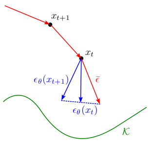
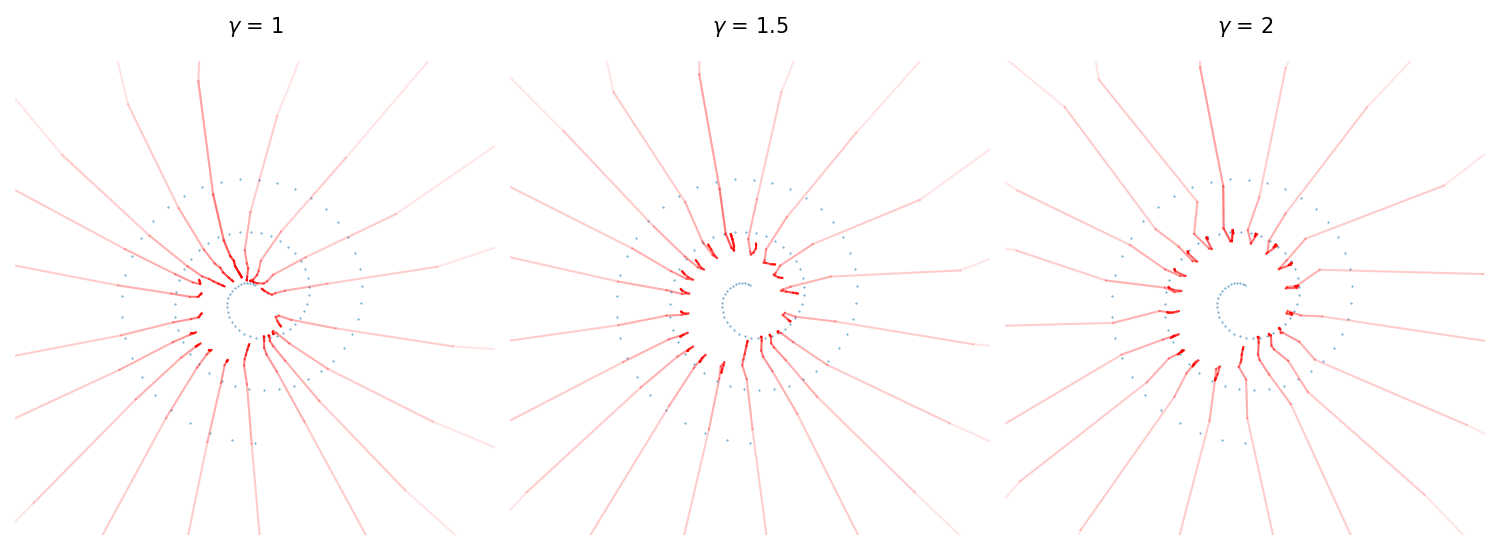
This leads to faster convergence compared to the DDIM sampler, as seen from the samples on our toy model lying closer to the original data.

Compared to the default DDIM sampler, our sampler can be interpreted as adding momentum, causing the trajectory to potentially overshoot but converge faster.

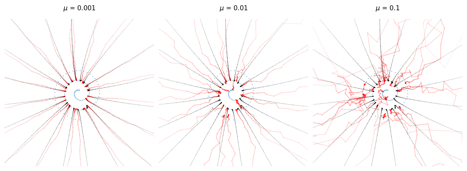
Empirically, adding noise during the generation process also improves the sampling quality. In order to do so while sticking to our original \(\sigma_t\) schedule, we need to denoise to a smaller \(\sigma_{t'}\) then add back noise \(w_t \sim N(0, I)\).

If we assume that \(\mathop{\mathbb{E}}\norm{w_t}^2 = \norm{\epsilon_\theta(x_t, \sigma_t)}^2\), we should choose \(\eta\) so that the norm of the update is constant in expectation. This leads to the choice of \(\sigma_{t-1} = \sigma_t^\mu \sigma_{t'}^{1-\mu}\) where \(0 \le \mu < 1\) (by definition, \(\sigma_{t'} \le \sigma_{t-1} \le \sigma_t\)), and \(\eta = \sqrt{\sigma_{t-1}^2 - \sigma_{t'}^2}\). When \(\mu = \frac{1}{2}\), we exactly recover the DDPM sampler (see Appendix A of our paper for a derivation).

Our gradient estimation update can be combined with adding noise during sampling. In summary, our full update step is

The full sampler that generalizes DDIM (gam=1, mu=0), DDPM (gam=1, mu=0.5) and our gradient estimation sampler (gam=2, mu=0) is implemented below.

@torch.no_grad()
def samples(model      : nn.Module,
            sigmas     : torch.FloatTensor, # Iterable with N+1 values for N sampling steps
            gam        : float = 1.,        # Suggested to use gam >= 1
            mu         : float = 0.,        # Requires mu in [0, 1)
            xt         : Optional[torch.FloatTensor] = None,
            batchsize  : int = 1):
    xt = model.rand_input(batchsize) * sigmas[0]
    eps = None
    for i, (sig, sig_prev) in enumerate(pairwise(sigmas)):
        eps, eps_prev = model(xt, sig.to(xt)), eps
        eps_av = eps * gam + eps_prev * (1-gam)  if i > 0 else eps
        sig_p = (sig_prev/sig**mu)**(1/(1-mu)) # sig_prev == sig**mu sig_p**(1-mu)
        eta = (sig_prev**2 - sig_p**2).sqrt()
        xt = xt - (sig - sig_p) * eps_av + eta * model.rand_input(batchsize).to(xt)
        yield xt

Large-scale examples

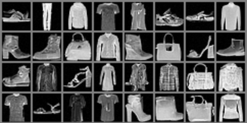
The training code above not only works for our toy dataset, they can also be used to train image diffusion models from scratch. See this example for an example of training on the FashionMNIST dataset to get a second-place FID score on this leaderboard:

The sampling code works without modifications to sample from state-of-the-art pretrained latent diffusion models:

schedule = ScheduleLDM(1000)
model    = ModelLatentDiffusion('stabilityai/stable-diffusion-2-1-base')
model.set_text_condition('An astronaut riding a horse')
*xts, x0 = samples(model, schedule.sample_sigmas(50))
decoded  = model.decode_latents(x0)

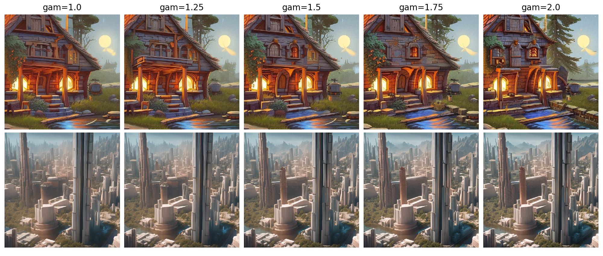
We can visualize the different effects of our momentum term \(\gamma\) on high resolution text-to-image generation.

Other resources

Also recommended are the following blog posts on diffusion models:

1. What are diffusion models introduces diffusion models from the discrete-time perspective of reversing a Markov process
2. Generative modeling by estimating gradients of the data distribution introduces diffusion models from the continuous time perspective of reversing a stochastic differential equation
3. The annotated diffusion model goes over a pytorch implementation of a diffusion model in detail

Citation

If you found this blog useful, please consider citing our paper:

@article{permenter2023interpreting,
  title={Interpreting and improving diffusion models using the euclidean distance function},
  author={Permenter, Frank and Yuan, Chenyang},
  journal={arXiv preprint arXiv:2306.04848},
  year={2023}
}